UniQuant 🧬
🧰 Name: Universal Quantile-Based Transcriptome Integration (R package)
📝 Note: UniQuant is a dynamic quantile normalization method for cross-platform heterogeneous data that effectively integrates RNA expression data from different platforms, batches, and formats. UniQuant eliminates batch effects and background differences between datasets, thereby generating more accurate and reliable integrated data, significantly improving the accuracy, reliability, and versatility of data analysis. The datasets integrated based on UniQuant can be used for building disease diagnosis models, molecular classification, survival analysis, differential gene expression analysis, and more.
✍️ Author: Huanhou Su
Quick run 🚀
##### 1. Quantile score
## Prepare raw data
# ls_datasset: Name of the dataset.
# df_raw: Raw expression data, with genes as rows and samples as columns.
# dataset_type: 'Training' or 'Validation'.
# df_Disease: The first column is the sample name, the second column is the disease status ('No' represents non-diseased samples, 'Yes' represents diseased samples). If survival information is available, the third column is the survival outcome (0 represents survival, 1 represents death), and the fourth column is the follow-up time (in months). Non-diseased samples do not need to have survival information filled in.
Quantile_score(ls_datasset, df_raw, dataset_type, df_Disease)

##### 2. Select the genes of interest
# Identify the top 1000 hypervariable genes from independent datasets and select those expressed across datasets.
rst_Hype = UniQuant_Hypervariable_gene(n_hypervariable_gene = 1000)
interest_gene = rst_Hype$Gene

##### 3. Training the diagnostic model
# Use the interest genes to identify disease-related genes.
rst_dg = UniQuant_Disease_gene(ls_gene = interest_gene)
Disease_gene = rst_dg$Disease_gene

# Train the diagnostic model using the identified disease-related genes.
rst_Training = UniQuant_Model_Training(ls_gene = Disease_gene)

##### 4. Validation of the diagnostic model
rst_Validation = UniQuant_Model_Validation()

##### 5. Molecular classification
# Perform molecular classification based on the selected genes of interest and classify into 3 groups.
rst_Class = UniQuant_Class(ls_gene = interest_gene, n_Class = 3)

##### 6. Subsequent analyses
# Perform additional analyses such as survival analysis, differential gene expression analysis, and enrichment analysis.
# These steps may follow depending on your dataset and goals.
Comprehensive Guide 📖
0️⃣ Setting
library(UniQuant);library(ggplot2); library(edgeR); library(pROC); library(stringr)

dir_main = getwd()
dir_in = file.path(dir_main, '0.raw')
dir_dataset = file.path(dir_main, 'UniQuant', 'dataset'); if(!dir.exists(dir_dataset)) dir.create(dir_result, recursive = TRUE)
dir_result = file.path(dir_main, 'UniQuant', 'result'); if(!dir.exists(dir_result)) dir.create(dir_result, recursive = TRUE)
setwd(dir_main); set.seed(100)
1️⃣ Quantile score
##### Converts raw expression data of a dataset into quantile-based scores and organizes the disease status of the samples.
#### Training set
ls_datassets = c('GSE6764', 'GSE14520', 'GSE17856', 'GSE57957', 'GSE36376','GSE102079', 'GSE54236', 'GSE36411', 'GSE22058')

for (ls_datasset in ls_datassets){
  df_raw = readRDS(file.path(dir_in, paste0(ls_datasset, '_Expression.rds')))
  df_Disease = readRDS(file.path(dir_in, paste0(ls_datasset, '_Disease.rds')))
  Quantile_score(ls_datasset, df_raw, "Training", df_Disease)
}


#### Validation set
ls_datassets = c('PMID31585088', 'PMID35382356', 'GSE77314', 'GSE76427','GSE25097', 'GSE63898', 'GSE39791', 'GSE144269','GSE114564', 'GSE14811')

for (ls_datasset in ls_datassets){
  df_raw = readRDS(file.path(dir_in, paste0(ls_datasset, '_Expression.rds')))
  df_Disease = readRDS(file.path(dir_in, paste0(ls_datasset, '_Disease.rds')))
  Quantile_score(ls_datasset, df_raw, "Validation", df_Disease)
}
⭕ You can also transform individual datasets.
ls_datasset = 'GSE36376'
df_raw = readRDS(file.path(dir_in, paste0(ls_datasset, '_Expression.rds')))
df_Disease = readRDS(file.path(dir_in, paste0(ls_datasset, '_Disease.rds')))
Quantile_score(ls_datasset, df_raw, "Validation", df_Disease)
⭕ The data format of the raw gene expression data is as follows.
df_raw[1:4, 1:4]
| GSM890128 | GSM890129 | GSM890130 | GSM890131 | |
|---|---|---|---|---|
| EEF1A1 | 14.054179 | 14.395189 | 14.349301 | 14.183636 |
| LOC643334 | 6.543733 | 6.399822 | 6.391479 | 6.190396 |
| SLC35E2 | 6.065169 | 6.172510 | 5.957617 | 5.980207 |
| LOC642820 | 6.862825 | 6.699461 | 6.726557 | 6.664170 |
⭕ The data format of the transformed gene expression data is as follows.
| GSE36376@GSM890128 | GSE36376@GSM890129 | GSE36376@GSM890130 | GSE36376@GSM890131 | |
|---|---|---|---|---|
| EEF1A1 | 4 | 9 | 8 | 6 |
| LOC643334 | 10 | 8 | 8 | 4 |
| SLC35E2 | 4 | 7 | 2 | 2 |
| LOC642820 | 9 | 5 | 6 | 4 |
⭕ The data format for the disease status of the samples is as follows.
print(rbind(head(df_Disease, 4), tail(df_Disease, 4)))
| Sample | Disease |
|---|---|
| GSM890128 | No |
| GSM890129 | No |
| GSM890130 | No |
| GSM890131 | No |
| GSM890557 | Yes |
| GSM890558 | Yes |
| GSM890559 | Yes |
| GSM890560 | Yes |
⭕
If your samples contain survival information, you can add columns for survival status (Outcome: 0 represents survival, 1 represents death) and survival time (Time: months).Note that only diseased samples require the addition of survival information.
ls_datasset = 'GSE14520'
df_Disease = readRDS(file.path(dir_in, paste0(ls_datasset, '_Disease.rds')))
head(df_Disease, 4)
| Sample | Disease | Outcome | Time |
|---|---|---|---|
| GSM362958 | Yes | 1 | 28.2 |
| GSM362959 | Yes | 1 | 9.5 |
| GSM362960 | Yes | 0 | 66.1 |
| GSM362961 | No |
2️⃣ Select the genes of interest
# Select the hypervariable genes that are expressed across the majority of the datasets.
rst_Hype = UniQuant_Hypervariable_gene(n_hypervariable_gene = 1000, dataset_threshold = 0.7)
interest_gene = rst_Hype$Gene

interest_gene
 [1] "ACSL4"   "AFP"     "AKR1B10" "ALDH3A1" "APOA4"   "APOF"    "C7"      "C9"      "CCL19"
[10] "CCL20"   "COL1A1"  "CRP"     "CTHRC1"  "CYP1A2"  "CYP3A4"  "DCN"     "DHRS2"   "DKK1"
[19] "DLK1"    "EPCAM"   "FCN3"    "FOS"     "FOSB"    "GPC3"    "GPR88"   "HAMP"    "HSD11B1"
[28] "IFI27"   "LCN2"    "LUM"     "MME"     "MMP7"    "MT1M"    "MUC13"   "MYH4"    "NQO1"
[37] "NTS"     "PAGE4"   "PEG10"   "PGC"     "PLA2G2A" "REG3A"   "RELN"    "S100P"   "SDS"
[46] "SLC22A1" "SLPI"    "SPINK1"  "SPP1"
⭕ You can enter other genes of interest, such as immune genes, metabolic genes, cell cycle genes, etc.
3️⃣ Training the diagnostic model
3.2 Train the model with disease-related genes
rst_Training = UniQuant_Model_Training(ls_gene = Disease_gene)

names(rst_Training)
[1] "Model_gene"     "AUC"            "Cutoff"         "Coefficient"
[5] "ROC_Model_plot" "ROC_Gene_plot"  "ROC_Model_data" "ROC_Gene_data"

# Model_gene: The genes used to construct the diagnostic model.
# AUC: The AUC value of the diagnostic model in the Training set.
# Cutoff: The sensitivity, specificity, and accuracy performance of the diagnostic model when the threshold is set to 0.5.
# Coefficient: The correlation coefficient of the model genes.
# ROC_Model_plot: The ROC curve plot of the diagnostic model in the Training set.
# ROC_Gene_plot: The ROC curve plot of the diagnostic model and its genes in the Training set.
# ROC_Model_data: The data used to plot the ROC curve of the diagnostic model in the Training set.
# ROC_Gene_data: The data used to plot the ROC curve of the diagnostic model and its genes in the Training set.

⭕
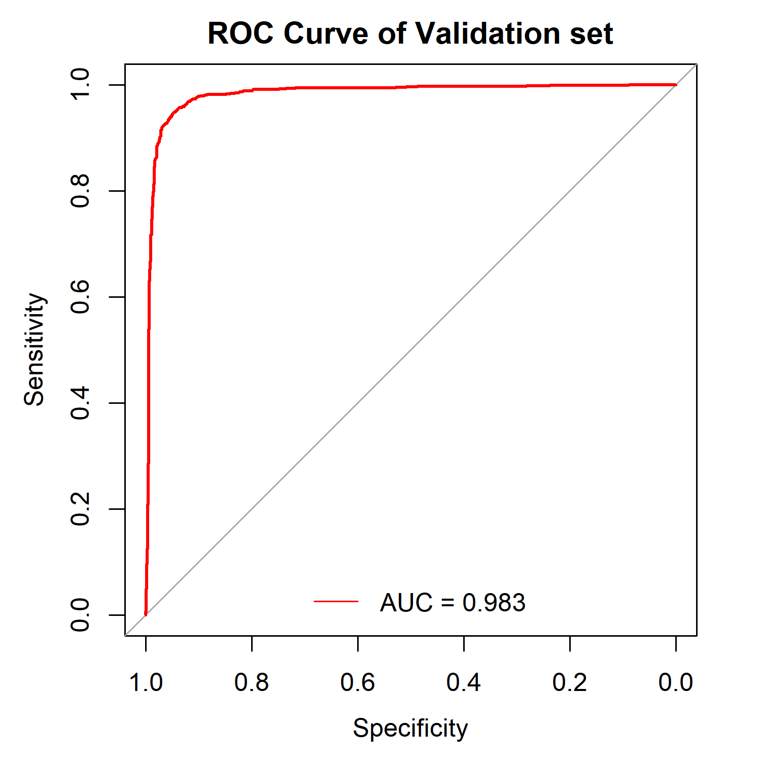
You can extract the data from rst_Training and plot the receiver operating characteristic (ROC) curve of the diagnostic model for the Training set.
res = rst_Training$ROC_Gene_data
p = ggroc(res, legacy.axes = TRUE)+
  geom_segment(aes(x = 0, xend = 1, y = 0, yend = 1), color="darkgrey", linetype=4)+
  theme_bw() +
  ggtitle("Training set")+
  theme(plot.title = element_text(hjust = 0.5,size = 25),
        axis.title.x = element_text(size = 20),
        axis.title.y = element_text(size = 20),
        axis.text=element_text(size=12,colour = "black"),
        panel.border = element_rect(color = "black", fill = NA, size = 1.5),

  ) + labs(colour = "Gene") +
  annotate("text", x=0.50, y=0.02, size = 7.5, label=paste("Model-AUC = ", round(res$Model$auc,3))); p

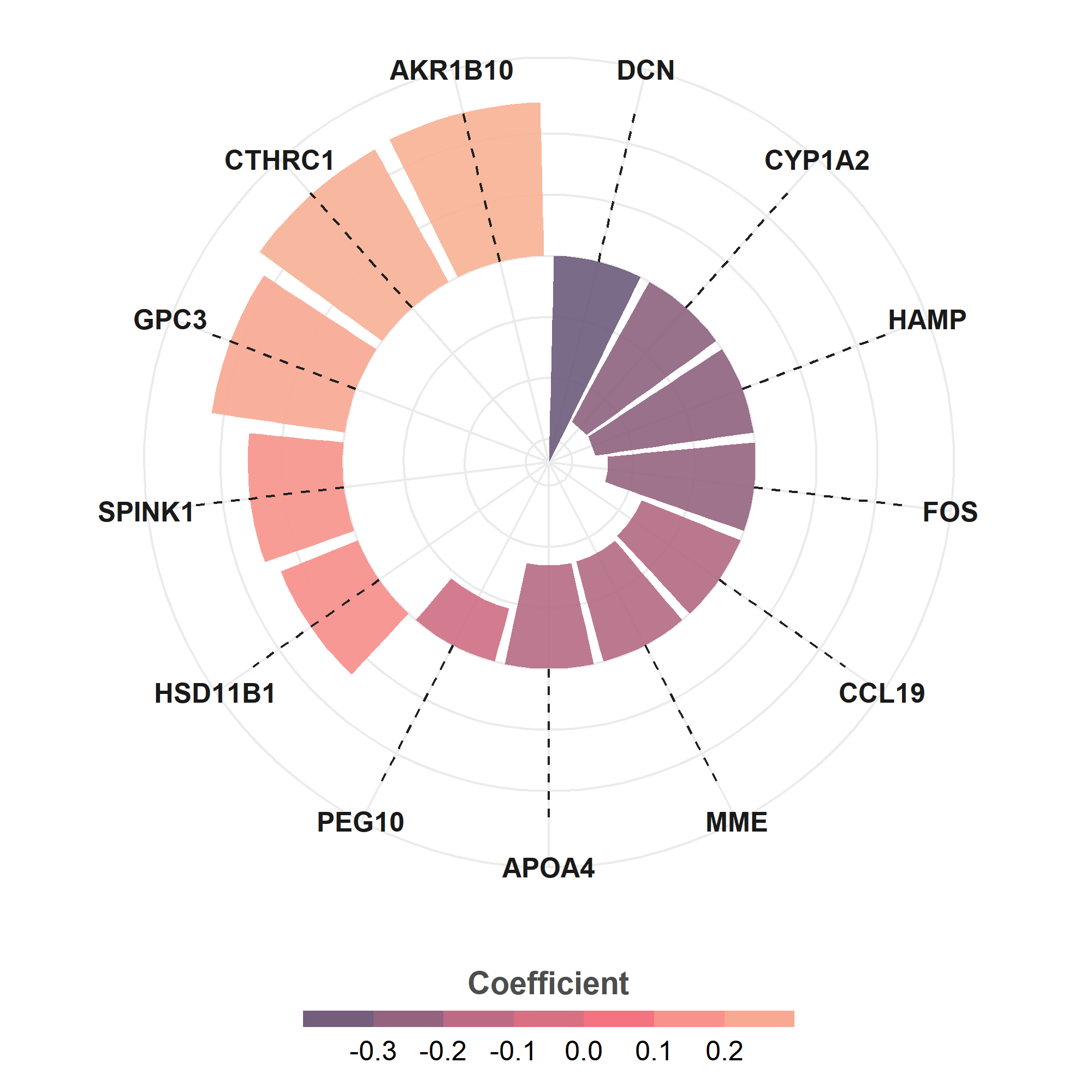
⭕ View the model genes and their corresponding coefficients.
rst_Training$Coefficient
| gene | coefficient |
|---|---|
| DCN | -0.33802661 |
| CYP1A2 | -0.26176605 |
| HAMP | -0.26145613 |
| FOS | -0.24085125 |
| CCL19 | -0.17432534 |
| MME | -0.16998127 |
| APOA4 | -0.16885766 |
| PEG10 | -0.08975637 |
| HSD11B1 | 0.13580332 |
| SPINK1 | 0.15481402 |
| GPC3 | 0.21975622 |
| CTHRC1 | 0.24801502 |
| AKR1B10 | 0.25147663 |
⭕ You can extract the model genes and their corresponding coefficients, and visualize the output.
df_plot = rst_Training$Coefficient
df_plot$gene = df_plot$gene
df_plot$coefficient = round(df_plot$coefficient, 3)


p1 = ggplot(df_plot) +
  geom_col(aes(x = reorder(str_wrap(gene, 8), coefficient),
               y = coefficient, fill = coefficient),
          position = "dodge2",
          show.legend = TRUE, alpha = .9
          ) +
  geom_segment(aes(
      x = reorder(str_wrap(gene, 8), coefficient), y = 0,
      xend = reorder(str_wrap(gene, 8), coefficient), yend = max(coefficient)),
      linetype = "dashed", color = "gray12") + coord_polar(); p1

p2 = p1 +
  scale_fill_gradientn(
    "Coefficient",
    colours = c( "#6C5B7B","#C06C84","#F67280","#F8B195")
  ) +
  guides(
    fill = guide_colorsteps(
    barwidth = 15, barheight = .5, title.position = "top", title.hjust = .5
    )) + theme_minimal()+
  theme(
    axis.title = element_blank(),
    axis.ticks = element_blank(),
    axis.text.y = element_blank(),
    axis.text.x = element_text(color = "gray10", size = 12, face = "bold"),
    legend.position = "bottom",
    legend.title = element_text(color = "gray30",size = 14, face = "bold"),
    legend.text = element_text(size = 12)
  ); p2
4️⃣ Validation of diagnostic model
rst_Validation = UniQuant_Model_Validation()

names(rst_Validation)
[1] "AUC"            "Cutoff"         "ROC_Model_plot"
[4] "ROC_Gene_plot"  "ROC_Model_data" "ROC_Gene_data"

# AUC: The AUC value of the diagnostic model in the Validation set.
# Cutoff: The sensitivity, specificity, and accuracy performance of the diagnostic model when the threshold is set to 0.5.
# ROC_Model_plot: The ROC curve plot of the diagnostic model in the Validation set.
# ROC_Gene_plot: The ROC curve plot of the diagnostic model and its genes in the Validation set.
# ROC_Model_data: The data used to plot the ROC curve of the diagnostic model in the Validation set.
# ROC_Gene_data: The data used to plot the ROC curve of the diagnostic model and its genes in the Validation set.
⭕
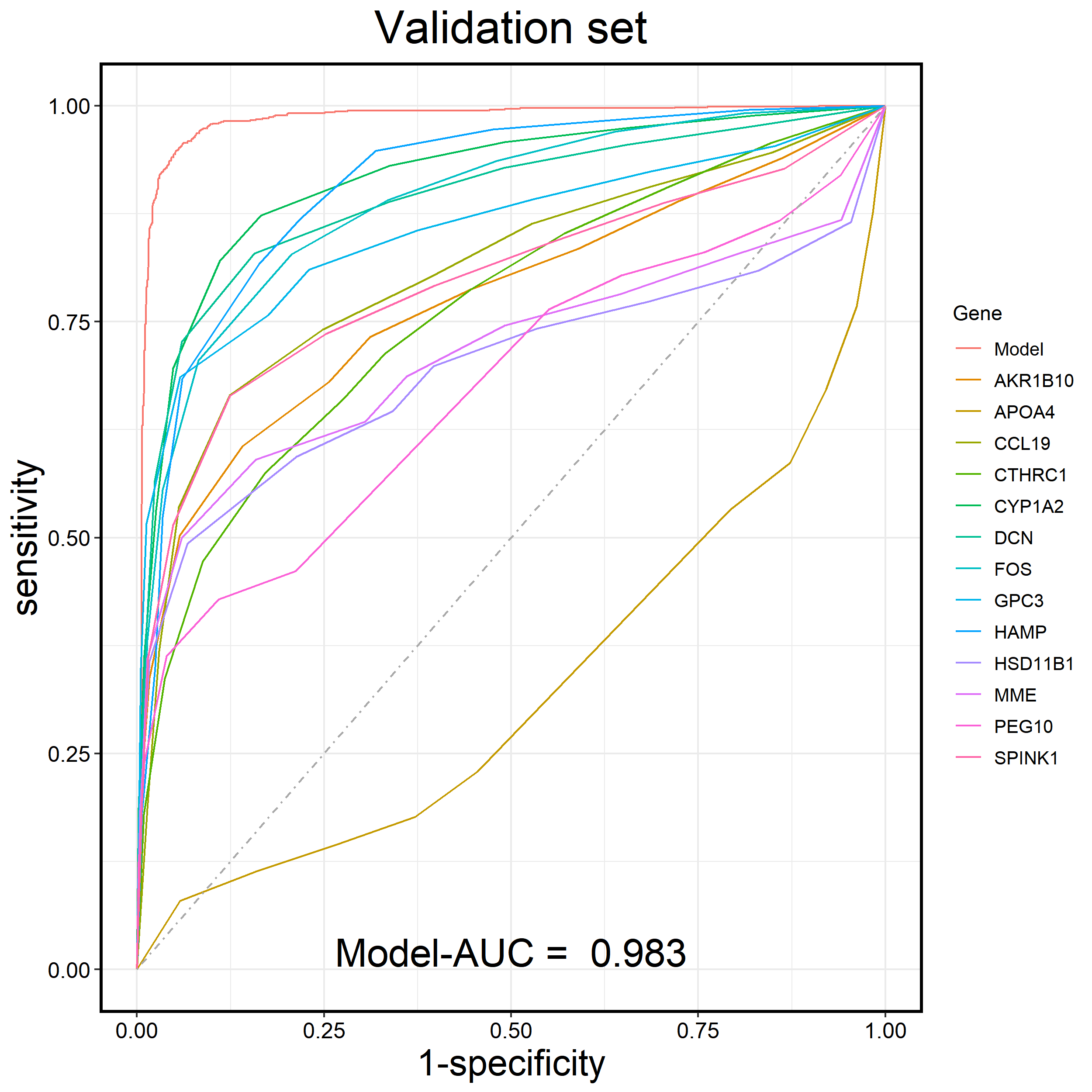
You can extract the data from rst_Validation and plot the receiver operating characteristic (ROC) curve of the diagnostic model for the Validation set.
rst_Validation$ROC_Gene_plot
5️⃣ Molecular classification
5.1 Classification
# Perform molecular classification of disease samples based on the integrated dataset.
rst_Class = UniQuant_Class(ls_gene = interest_gene, n_Class = 3)
df_Class = rst_Class$df_Class

# Count the number of samples for each molecular classification
rst_Class$df_Class_table
Class_1 Class_2 Class_3
    570     690     708
⭕ View the molecular classification results of all samples.
head(df_Class)
| Sample | Class |
|---|---|
| GSE102079@GSM2723193 | Class_1 |
| GSE102079@GSM2723195 | Class_2 |
| GSE102079@GSM2723197 | Class_2 |
| GSE102079@GSM2723198 | Class_1 |
| GSE102079@GSM2723199 | Class_3 |
| GSE102079@GSM2723200 | Class_2 |
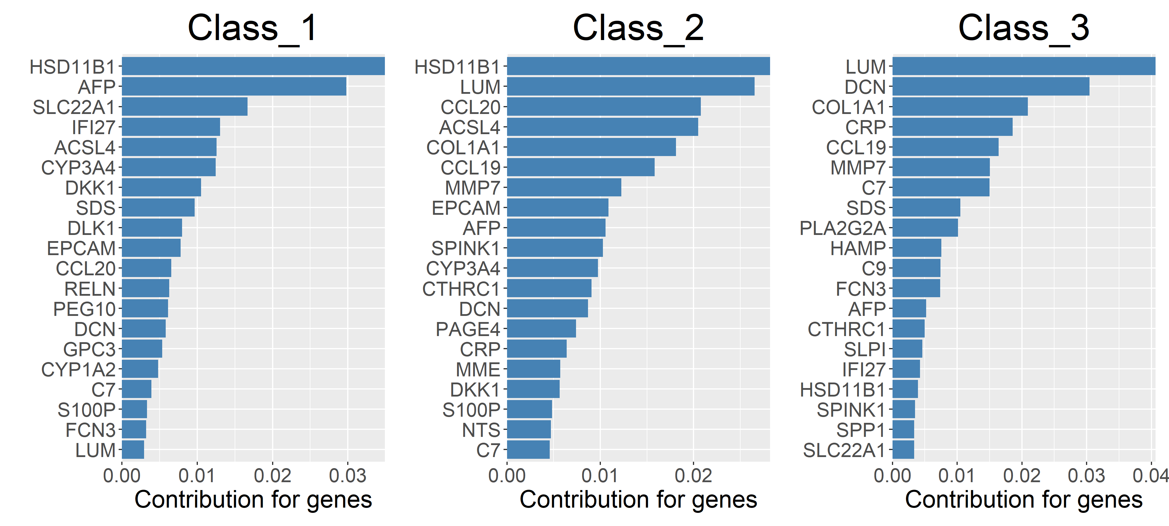
5.2 Gene contribution
⭕ Using machine learning methods to calculate the contribution of genes to molecular classification.
# num_Top: Number of top genes to display based on their contribution score.
# n_Train: Number of classification training tasks.
rst_Contribution = UniQuant_Class_Contribution(num_Top = 20, n_Train = 2)

rst_Contribution$Acc
    Class Accuracy
  Class_1    0.984
  Class_2    0.990
  Class_3    0.983
# Display the contribution of genes to molecular typing in a table format
head(rst_Contribution$Contribution)
| Gene | Class_1 | Class_2 | Class_3 |
|---|---|---|---|
| ACSL4 | 0.0125754340 | 0.0204913958 | 0.0018271964 |
| AFP | 0.0297757726 | 0.0105659208 | 0.0051961789 |
| AKR1B10 | 0.0003743662 | 0.0006829170 | 0.0010541345 |
| ALDH3A1 | 0.0016005614 | 0.0018106727 | 0.0007021926 |
| APOA4 | 0.0003649859 | 0.0011380439 | 0.0006137823 |
| APOF | 0.0021530311 | 0.0007603114 | 0.0023867149 |
# Display the contribution of genes to molecular typing in a bar chart format
rst_Contribution$Plot_bar
# Display the contribution of genes to molecular typing in a heatmap format
rst_Contribution$Plot_heatmap

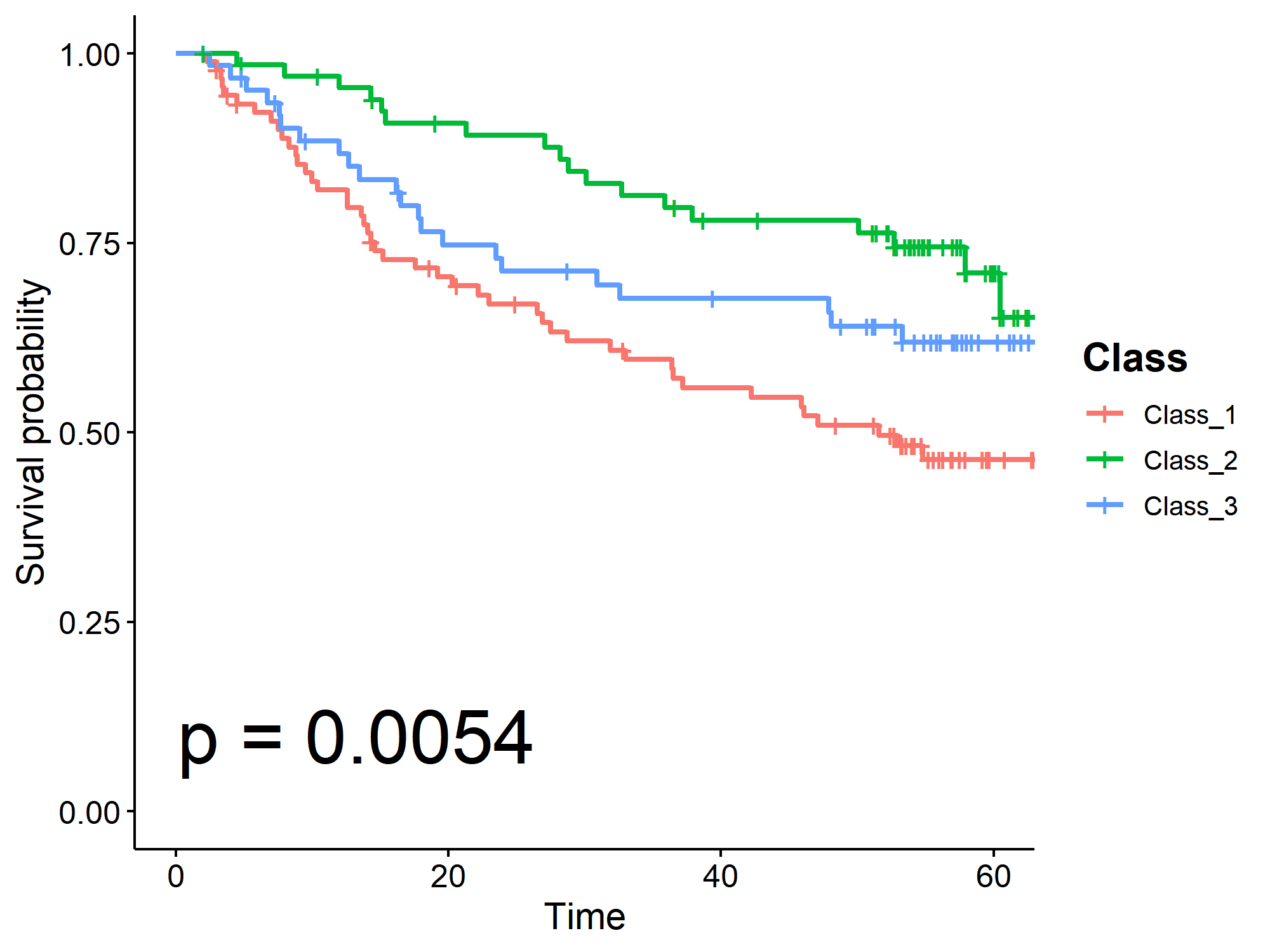
5.3 Survival analysis
⭕ Analyze the impact of molecular classification on patient survival outcomes in the specified dataset.
library(survival); library(survminer)

ls_dataset = 'GSE14520'
df_Disease = readRDS(file.path(dir_dataset, paste0(ls_dataset, '@Disease.rds')))
df_Class = readRDS(file.path(dir_result, 'df_Class.rds'))

df_Disease = df_Disease[!is.na(df_Disease$Time),]
df_Class_tmp = df_Class[df_Class$Sample %in% df_Disease$Sample,]
df_Disease_Class = merge(df_Disease, df_Class_tmp, by = 'Sample')
unique_Class = as.character(sort(unique(df_Disease_Class$Class)))

sfit = survfit(Surv(Time, Outcome)~Class, data = df_Disease_Class)
p = ggsurvplot(sfit, pval = TRUE, data = df_Disease_Class, risk.table = FALSE,
                legend.title = "Class",
                legend.labs = unique_Class,
                legend = "right",
                pval.size = 10,
                pval.coord = c(0.1,0.1),
                palette = c("#F8766D", "#00BA38", "#619CFF")
)

p$plot = p$plot + theme(legend.title = element_text(face = "bold", size = 15)); p
6️⃣ Differential gene expression (DEG) analysis.
6.1 DEG:Disease
# Perform DEG analysis based on the disease status of the samples
rst_DEG_Disease = UniQuant_DEG_Disease(dataset_threshold = 0.7)
df_DEG_Disease = rst_DEG_Disease$DEG

head(df_DEG_Disease)
| Gene | LogFC | logCPM | LR | PValue | FDR |
|---|---|---|---|---|---|
| CAP2 | 1.134334 | 6.434386 | 3076.955 | 0 | 0 |
| ASPM | 1.129646 | 6.434048 | 3052.996 | 0 | 0 |
| TOP2A | 1.124791 | 6.434128 | 3028.964 | 0 | 0 |
| PRC1 | 1.116258 | 6.433803 | 2987.175 | 0 | 0 |
| RACGAP1 | 1.112615 | 6.434054 | 2969.149 | 0 | 0 |
| CENPF | 1.111725 | 6.433586 | 2963.983 | 0 | 0 |
6.2 DEG:Class
# Perform DEG analysis based on the molecular classification of the samples
rst_DEG_Class = UniQuant_DEG_Class(
  input_Class = rst_Class$df_Class,
  Class_test = 'Class_3',
  Class_control = c('Class_1', 'Class_2'),
  dataset_threshold = 0.7)

head(df_DEG_Class)
| Gene | LogFC | logCPM | LR | PValue | FDR |
|---|---|---|---|---|---|
| FGFR3 | 0.860094 | 6.350244 | 556.9723 | 3.830429e-123 | 1.962663e-120 |
| PDE9A | 0.857775 | 6.367620 | 503.9286 | 1.327970e-111 | 3.766691e-109 |
| AFP | 0.827938 | 6.476032 | 580.9512 | 2.329059e-128 | 1.541449e-125 |
| PEG3 | 0.780960 | 6.214317 | 330.6309 | 7.004662e-74 | 5.705746e-72 |
| PPP1R9A | 0.750667 | 6.433330 | 395.2754 | 5.880676e-88 | 7.983646e-86 |
| EPCAM | 0.746381 | 6.243183 | 300.1526 | 3.051573e-67 | 1.923460e-65 |
⭕ After obtaining the DEGs, further analyses can be conducted, such as protein-protein interaction network, Gene Set Enrichment Analysis (GSEA), transcription factor analysis, etc.
6️⃣ 7️⃣ 8️⃣ 9️⃣
All functions 🔧
Quantile_score
🚩 Converts raw expression data of a dataset into quantile-based scores and organizes the disease status of the samples.
| Parameter | Type | Description |
|---|---|---|
| dataset_name | Character | Name of the dataset. |
| dataset_expression | Data.frame | Raw expression data, with genes as rows and samples as columns. |
| dataset_type | Character | 'Training' or 'Validation'. |
| dataset_disease | Data.frame | The first column is the sample name, the second column is the disease status ('No' represents non-diseased samples, 'Yes' represents diseased samples). If survival information is available, the third column is the survival status (0 represents survival, 1 represents death), and the fourth column is the follow-up time (in months). Non-diseased samples do not need to have survival information filled in. |
UniQuant_Hypervariable_gene
🚩 Select the hypervariable genes that are expressed across the majority of the datasets.
| Parameter | Type | Description |
|---|---|---|
| n_hypervariable_gene | Integer | 1-3000. The number of hypervariable genes selected from each dataset. |
| dataset_threshold | Numeric | 0-1.0. The minimum proportion of datasets in which the selected genes must be expressed. |
UniQuant_Disease_gene
🚩 Select disease-related genes with high AUC from the Training set.
| Parameter | Type | Description |
|---|---|---|
| ls_gene | Vector | The vector containing multiple genes. |
| dataset_threshold | Numeric | 0-1.0. The minimum proportion of datasets in which the selected genes must be expressed. |
UniQuant_Model_Training
🚩 Build a disease diagnostic model using the integrated training dataset.
| Parameter | Type | Description |
|---|---|---|
| ls_gene | Vector | The vector containing multiple genes. |
UniQuant_Model_Validation
🚩 Analyze the performance of the disease diagnostic model using the integrated validation dataset.
UniQuant_Model_dataset_AUC
🚩 Analyze the diagnostic performance of the disease diagnostic model across all datasets.
UniQuant_Remove_dataset
🚩 Remove the specified dataset.
| Parameter | Type | Description |
|---|---|---|
| dataset_name | Character | Name of the dataset. |
UniQuant_Class
🚩 Perform molecular classification of disease samples based on the integrated dataset.
| Parameter | Type | Description |
|---|---|---|
| ls_gene | Vector | A vector containing a list of genes to be processed. |
| n_Class | Integer | The number of molecular classifications to be used. |
| method | Character | The method for classification, either 'CCP' or 'NMF'. |
UniQuant_Class_Contribution
🚩 Identifies the top contributing genes based on their importance in molecular classification.
| Parameter | Type | Description |
|---|---|---|
| num_Top | Integer | Number of top genes to display based on their contribution score. |
| n_Train | Integer | Number of classification training tasks. |
| reTrain | Logical | If TRUE, the tasks will be retrained. |
UniQuant_DEG_Disease
🚩 Perform differential gene expression analysis between disease and non-disease samples.
| Parameter | Type | Description |
|---|---|---|
| dataset_threshold | Numeric | 0-1.0. The minimum proportion of datasets in which the selected genes must be expressed. |
UniQuant_DEG_Class
🚩 Perform differential gene expression analysis between different molecular classification.
| Parameter | Type | Description |
|---|---|---|
| input_Class | Data.frame | The first column represents the samples, and the second column represents the molecular classification. |
| Class_test | Character | The target molecular classification for differential expression analysis. |
| Class_control | Vector | The contrast molecular classification for differential expression analysis. |
| dataset_threshold | Numeric | 0-1.0. The minimum proportion of datasets in which the selected genes must be expressed. |
UniQuant_dataset
🚩 View information about the dataset.
| Parameter | Type | Description |
|---|---|---|
| Sample | Logical | If TRUE, counts the number of diseased and non-diseased samples. |
Reference 🔖
Huanhou Su et al. Deciphering the Oncogenic Landscape of Hepatocytes through Integrated Single-Nucleus and Bulk RNA-Seq of Hepatocellular Carcinoma. Advanced Science. 2025. DOI: [10.1002/advs.202412944]